Vector data - styles

This section introduces more ways to style your vactor data, including adding colours and legends.

Example: Wind from Storm Ophelia (October 2017)

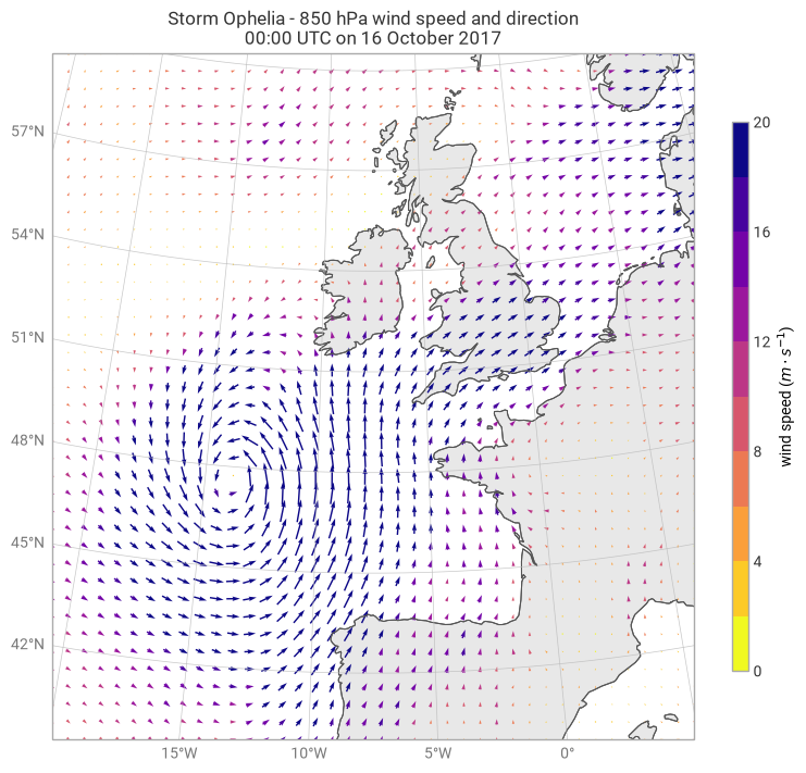
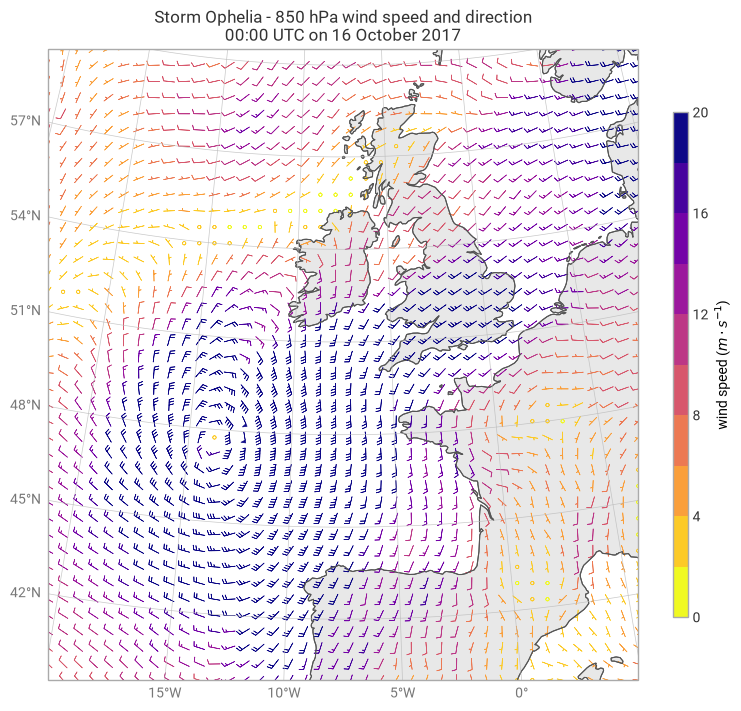
In this example, we will use sample wind data from Storm Ophelia, which impacted the UK in October 2017.

import earthkit.data as ekd

import earthkit.plots as ekp

data = ekd.from_source("sample", "storm_ophelia_wind_850.grib").to_fieldlist()
data.ls()

	parameter.variable	time.valid_datetime	time.base_datetime	time.step	vertical.level	vertical.level_type	ensemble.member	geography.grid_type
0	u	2017-10-16	2017-10-16	0 days	850	pressure	0	regular_ll
1	v	2017-10-16	2017-10-16	0 days	850	pressure	0	regular_ll

Passing a Style

We can plot our vector field with a Style, much like we can for contour and raster fields. This allows us to pass colour schemes, levels and units to apply to our vector fields.

style = ekp.styles.Style(
    colors="plasma_r",
    levels=range(0, 22, 2),
    units="m s-1",
)

(
    ekp
    .geo.quiver(data, style=style, domain=[-20, 5, 40, 60], legend=False)
    .legend(label="wind speed ({units})", location="right")
    .land()
    .coastlines()
    .gridlines()
    .title("Storm Ophelia - {vertical.level} hPa wind speed and direction\n{time:%H:%M UTC on %-d %B %Y}")
    .show()
)

<earthkit.plots.components.figures.Figure at 0x14e2d1490>

And you can of course do the same with barbs:

style = ekp.styles.Style(
    colors="plasma_r",
    levels=range(0, 22, 2),
    units="m s-1",
)

(
    ekp
    .geo.barbs(data, style=style, domain=[-20, 5, 40, 60], legend=False)
    .legend(label="wind speed ({units})", location="right")
    .land()
    .coastlines()
    .gridlines()
    .title("Storm Ophelia - {vertical.level} hPa wind speed and direction\n{time:%H:%M UTC on %-d %B %Y}")
    .show()
)

<earthkit.plots.components.figures.Figure at 0x16207b910>